# Dr. M. Baron, Statistical Machine Learning class, STAT-427/627

# RESAMPLING: JACKKNIFE and BOOTSTRAP

1. JACKKNIFE

# Package “bootstrap” has a jackknife tool. For example, here is a bias reduction for a sample variance.

# We’ll start with the biased version of a sample variance.

> variance.fn = function(X){ return( mean( (X-mean(X))^2 ) ) }

> variance.fn(mpg)

[1] 60.76274

# Use jackknife to correct its bias.

> install.packages(“bootstrap”)

> library(bootstrap)

> variance.JK = jackknife( mpg, variance.fn )

# This gives us the jackknife estimates of standard error and bias, as well as all estimates _(-i)

> names(variance.JK)

[1] "jack.se" "jack.bias" "jack.values" "call"

> variance.JK

$jack.se

[1] 3.741951

$jack.bias

[1] -0.1554034

$jack.values

[1] 60.84210 60.73524 60.84210 60.77598 60.81160 60.73524 60.68936 60.68936 60.68936 60.73524 60.73524 60.68936 60.73524 60.68936 60.91735 60.91278 60.84210 60.90280

[19] 60.88575 60.90142 60.91195 60.91735 60.91195 60.90142 60.90280 60.45457 60.45457 60.52096 60.38306 60.88575 60.86496 60.91195 60.86746 60.77598 60.81160 60.86746

[37] 60.84210 60.68936 60.68936 60.68936 60.68936 60.58222 60.63836 60.63836 60.84210 60.91278 60.86746 60.84210 60.91763 60.86496 60.80800 60.80800 60.77182 60.57584

[55] 60.88575 60.90142 60.91735 60.91195 60.91763 60.88770 60.90280 60.63836 60.68936 60.73524 60.68936 60.81160 60.52096 60.63836 60.58222 60.63836 60.86746 60.73524

[73] 60.63836 60.63836 60.68936 60.84210 60.91278 60.90280 60.90142 60.91278 60.86496 60.91763 60.86496 60.88575 60.63836 60.68936 60.63836 60.68936 60.73524 60.58222

[91] 60.63836 60.63836 60.68936 60.63836 60.58222 60.63836 60.84210 60.77598 60.84210 60.84210 60.91763 60.90142 60.52096 60.58222 60.63836 60.58222 60.84210 60.88770

[109] 60.90280 60.91278 60.84210 60.86746 60.90280 60.90142 60.73524 60.77598 60.83905 60.91735 60.88770 60.86746 60.73524 60.91735 60.88770 60.52096 60.88770 60.86746

[127] 60.73524 60.77182 60.90142 60.73052 60.91195 60.77598 60.77598 60.84210 60.77598 60.63836 60.68936 60.68936 60.68936 60.83905 60.90142 60.90142 60.77182 60.73052

[145] 60.86496 60.91735 60.90142 60.91735 60.90142 60.77182 60.86746 60.84210 60.73524 60.73524 60.77598 60.73524 60.77598 60.68936 60.81160 60.77598 60.73524 60.84210

[163] 60.90280 60.88770 60.63836 60.83905 60.91763 60.88770 60.91763 60.91735 60.91195 60.91735 60.84210 60.83905 60.86746 60.91763 60.91763 60.91278 60.91195 60.68409

[181] 60.86496 60.91195 60.91195 60.90142 60.88575 60.82749 60.77598 60.75625 60.71294 60.91278 60.91278 60.91735 60.91585 60.83905 60.91529 60.83905 60.68409 60.88770

[199] 60.84210 60.85542 60.82749 60.82416 60.73052 60.86496 60.89423 60.88770 60.63836 60.86746 60.86746 60.79444 60.79444 60.63836 60.63836 60.63836 60.75181 60.80800

[217] 60.51403 60.90732 60.65895 60.82749 60.81160 60.75625 60.73524 60.82749 60.89589 60.86746 60.85542 60.77598 60.75625 60.75625 60.77598 60.83905 60.91529 60.90142

[235] 60.90732 60.79055 60.65895 60.80800 60.79055 60.91278 60.90843 60.90843 59.92768 60.50757 60.69379 60.26550 60.50757 60.88590 60.87617 60.89113 60.87192 60.89589

[253] 60.89113 60.91113 60.89589 60.87617 60.89737 60.90019 60.85793 60.84486 60.87192 60.83349 60.84486 60.82749 60.80800 60.87600 60.88201 60.77567 60.90403 60.91799

[271] 60.91782 60.91761 60.89277 60.81160 60.90940 60.78352 60.75181 60.82416 60.90843 60.88406 60.91477 60.89113 60.89737 60.81160 60.83051 60.79444 60.84758 60.80827

[289] 60.75625 60.87192 60.85542 60.73488 60.62709 60.53311 60.87805 60.90835 60.91763 60.88201 60.91761 60.62160 60.60483 60.73919 60.42600 60.85521 60.84464 60.88930

[307] 60.65895 60.08238 60.36752 60.72611 60.43308 60.86496 60.89577 60.91627 60.86971 60.61606 60.81462 60.75997 60.44709 60.72165 59.54351 60.86727 60.14593 59.80304

[325] 59.89721 60.48787 60.80800 59.77073 60.64325 60.81462 60.69856 60.91798 60.57584 60.71256 60.88201 60.89263 60.90393 60.91813 60.80800 60.28981 60.29781 60.56989

[343] 60.71713 60.44709 60.39717 60.62709 60.59339 60.61047 60.81133 60.68409 60.64854 60.71256 60.68896 60.74766 60.86260 60.78322 60.90835 60.91668 60.91534 60.89263

[361] 60.89113 60.83051 60.86496 60.88575 60.63253 60.77182 60.83905 60.88575 60.91735 60.51403 60.44709 60.77182 60.37501 60.51403 60.51403 60.51403 60.63253 60.37501

[379] 60.73052 60.37501 60.91195 60.37501 60.90142 60.91278 60.73052 60.51403 60.88575 60.88575 59.83489 60.73052 60.86496 60.77182

# We can now calculate the jackknife variance estimator by the jackknife formula

> n* variance.fn(mpg) - (n-1)*mean(variance.JK$jack.values)

[1] 60.91814

# … or subtracting the bias from the original estimator

> variance.fn(mpg) - variance.JK$jack.bias

[1] 60.91814

# … and this is precisely the usual, unbiased version of the sample variance.

> var(mpg)

[1] 60.91814

2. BOOTSTRAP

(a) A simple example: use bootstrap to estimate the standard deviation of a sample median.

> B = 1000 # Number of bootstrap samples

> n = length(mpg) # Sample size (and the size of each bootstrap sample)

> median_bootstrap = rep(0,B) # Initiate a vector of bootstrap medians

> for (k in 1:B){ # Do-loop to produce B bootstrap samples.

+ b = sample( n, n, replace=TRUE ) # Take a random subsample of size n with replacement

+ median_bootstrap[k] = median( mpg[b] ) # Compute the sample median of each bootstrap subsample

+ }

> hist(median_bootstrap)

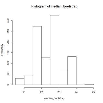
> median(mpg) # The actual sample median is 22.75; bootstrap medians range

[1] 22.75 # from 20.5 to 25.0.

> sd(median_bootstrap)

[1] 0.7661376 # The bootstrap estimator of SD(median) is 0.7661376.

(b) Bootstrap confidence interval

# The histogram above shows the distribution of a sample median. We can find its (α/2)-quantile and

(1-α/2)-quantile. They estimate the true quantiles that embrace the sample median with probability (1-α).

> alpha=0.05; quantile( median_bootstrap, alpha/2 )

2.5%

21

> quantile( median_bootstrap, 1-alpha/2 )

97.5%

24

# A bootstrap confidence interval for the population median is [21, 24].

(c) R package “boot”

# There is a special bootstrap tool in R package “boot”.

# To use it for the same problem, we define a function that computes a sample median for a given subsample…

> median.fn = function(X,subsample){

+ return(median(X[subsample]))

+ }

# For example, here is a sample median for a small subsample of size 10 without replacement…

> median.fn( mpg, sample(n,10) )

[1] 24.95

# If the subsample is the whole sample, with all its indices, we get our original sample median…

> median.fn( mpg, )

[1] 22.75

# Then we apply this function to many bootstrap samples (R is their number) and summarize the obtained statistics…

> library (boot)

> boot( mpg, median.fn, R=10000 )

ORDINARY NONPARAMETRIC BOOTSTRAP

Call:

boot(data = mpg, statistic = median.fn, R = 10000)

Bootstrap Statistics :

original bias std. error

t1* 22.75 -0.1406 0.7687722

# The bootstrap estimate of the standard deviation of a sample median is 0.7687722, and the bootstrap estimate of the bias is -0.1406. If we run the same command again, we might get somewhat different estimates, because the bootstrap method is based on random resampling.

> boot( mpg, median.fn, R=10000 )

original bias std. error

t1* 22.75 -0.13368 0.7727318

> boot( mpg, median.fn, R=10000 )

original bias std. error

t1* 22.75 -0.13437 0.7617304

(d) Another problem – find a bootstrap estimate of the standard deviation of each regression coefficient

# Define a function returning regression intercept and slope…

> slopes.fn = function( dataset, subsample ){

+ reg = lm( mpg ~ horsepower, data=dataset[subsample, ] )

+ beta = coef(reg)

+ return(beta)

+ }

> boot( Auto, slopes.fn, R=10000 )

Bootstrap Statistics :

original bias std. error

t1* 39.9358610 0.0329999048 0.857890744

t2* -0.1578447 -0.0003929433 0.007444107

# We got bootstrap estimates, Std(intercept) = 0.85789, Std(slope) = 0.007444.

# Actually, this can be obtained easily, and without bootstrap…

> summary( lm( mpg ~ horsepower, data=Auto ) )

Coefficients:

Estimate Std. Error t value Pr(>|t|)

(Intercept) 39.935861 0.717499 55.66 <2e-16 ***

horsepower -0.157845 0.006446 -24.49 <2e-16 ***

# But…. Why are the bootstrap estimates of standard errors higher than the ones obtained by regression formulae? Random variation due to bootstrapping? Let’s try bootstrap a few more times.

> boot( Auto, slopes.fn, R=10000 )

original bias std. error

t1* 39.9358610 0.0366632516 0.864274619

t2* -0.1578447 -0.0003676081 0.007459809

> boot( Auto, slopes.fn, R=10000 )

original bias std. error

t1* 39.9358610 0.024793987 0.866532993

t2* -0.1578447 -0.000309597 0.007501155

> boot( Auto, slopes.fn, R=10000 )

Bootstrap Statistics :

original bias std. error

t1* 39.9358610 0.0411404502 0.868404735

t2* -0.1578447 -0.0004208256 0.007500111

# A comment about discrepancy with the standard estimates. Bootstrap estimates are pretty close to each other. They should be, because each of them is based on 10,000 bootstrap samples. However, the bootstrap standard errors of slopes are still a little higher than the estimates obtained by the standard regression analysis. The book explains this phenomenon by a number of assumptions that the standard regression requires. In particular, nonrandom predictors X and a constant variance of responses Var(Y) = σ². Bootstrap is a nonparametric procedure, it is not based on any particular model. Thus, it can account for the variance of predictors. Here, “horsepower” is the predictor, and it is probably random.

Since some of the standard regression assumptions are questionable here, the bootstrap method for estimating standard errors is more reliable.